RUCOOL Updates: April & May, 2020

Despite the COVID-19, RUCOOL remains active.  Core technologies (storm gliders and HF Radar) were deemed critical research tools based on national security requirements and continue to be supported. These activities are guided by an operations plan that maintains recommended COVID best practices.

State

• On June 3, Rutgers scientists observed the ocean and atmospheric response to a derecho that passed through NJ.  The RUCOOL meteorological tower in Tuckerton NJ recorded a peak wind gust of 54 mph alongside a 21-degree temperature drop in only 15 minutes.  The Rutgers HF-Radar station detected a meteotsunami hitting New Jersey.
• The 4-H STEM program continues to support summer learning with the STEM Blog and 4-H from Home programs.
• RUCOOL took delivery of RU34, a new Slocum glider purchased for the Orsted ECO-PAM project. The glider is equipped with the passive acoustic sensor designed track vocalizing right whales in the area within and around Orsted’s Ocean Wind lease area off of NJ. The R/V Rutgers was formally approved by Orsted’s health and safety department and can now be used for Orsted-RU collaborative work.
• Through NSF funding, We took deliver a multi-frequency active BioSonics system for continuously measuring fish and zooplankton at the RUMFS which will be coupled to a SubSea hydrophone to track marine mammals.
• The first two Masters of Operational Oceanography have formalized their thesis.  One of the students has been hired by NOAA even before graduation.

National

• The hurricane season is upon us and the RUCOOL glider team is organizing a fleet of glider deployments throughout the Mid Atlantic, funded by NOAA. Partners this year include UMass Dartmouth, Virginia Institute of Marine Science, the University of Delaware, SUNY Stony Brook, Monmouth University and the US Navy. RUCOOL will be deploying and recovering the Navy gliders.
• RUCOOL presented overviews of Glider and HR-Radar to members of mid-Atlantic US congress (Senate and House). They reviewed the technologies and their critical needs to support NWS hurricane forecast improvements, USCG search and rescue, and the newly developed wave forecasts.
• Scott Glenn joined Mark Abbott (Director and President of Woods Hole Oceanographic Institution) and John Delaney (Professor Emeritus, University of Washington) as new members of the National Academies of Science, Engineering and Medicine (NASEM) Ocean Studies Board (OSB). The NASEM OSB is the official U.S. Committee for the U.N. Decade of Ocean Science for Sustainable Development is charged with coordinating the U.S. contributions to the U.N. Decade.
• Scott Glenn began posting to the RUCOOL Hurricane Blog on May 15 for the 2020 hurricane season.  The blog site (link here) has been circulated within NOAA leadership circles and was distributed through the US IOOS Eyes-on-the-Ocean as one of their recommended data resources.

• The RIOS program together with the Data Labs project team launched a new virtual REU program for 15 undergraduates from around the country in rapid response to COVID 19.  See https://datalab.marine.rutgers.edu/2020-virtual-reu/.
• The RUCOOL Engagement and Outreach team is completing a four part professional development program for 8 early career polar scientists. They will create new curriculum for presentation to the Newark Public School District this summer as a summer enrichment program.  Our focus will be on building student’s polar literacy and data skills.  See polar-ice.org

International

• Travis Miles was invited to be on the steering committee for the Interagency Ocean Observing Committee Underwater Glider User Group. This team is slated to lead the international efforts on underwater glider operations, science, QA/QC, best practices, organizing international meetings and driving the future development of these gliders and associated instrumentation.
• IOCARIBE, the Global Ocean Observing System’s (GOOS) Implementing Organization for the Caribbean Sea, voted to endorse the Caribe Corredores plan prepared by Scott Glenn, Doug Wilson of Ocean and Coastal Observing -Virgin Islands (OCO-VI) and Tony Knap of Texas A&M University as a component of their contribution to the UN Decade of Ocean Science for Sustainable Development.  The plan proposes to implement the HF Radar and glider observational components contained in the Rutgers MacArthur pre-proposal.
• Scott Glenn was asked to join the NOAA Global Ocean Monitoring and Observation (GOMO) Program, specifically to work on their Extreme Events Team. The team’s first task is to plan the integrated ocean/atmosphere hurricane experiment for the 2021 season.
• NSF is moving ahead to grant the Rutgers Palmer LTER project a field season. Given disruptions associated with COVID, this will likely be one of the few field efforts in Southern Ocean this coming year supported by the United States.  Scientists will have to take a 2-week quarantine onboard the ship prior to the deployment.

Student Awards

• Congratulations to Michael Brown for his successful PhD defense.  His thesis was focused on the “Drivers of phytoplankton dynamics, and corresponding impacts on biogeochemistry, along the West Antarctic Peninsula”.  His thesis examined how the physics drives the phytoplankton dynamics and the consequences on the biogeochemistry.  Congrats to Mike for an excellent piece of work!
• Emily Slesinger will receive $1000 from the George Burlew Scholarship program (Manasquan River Marline & Tuna Club).  Her research focus is on the optimal thermal and oxygen niches for black sea bass and use the information to better understand their potential population trajectories in the future.
• Hailey Conrad is a member of the Rutgers Honors College. She began doing research her freshman year with DMCS by volunteering in the OOI Hydrothermal Vent Lab where she reconstructed time lapse video of hydrothermal vents. She working with the Schofield lab in Antarctica to monitor phytoplankton populations and working as an Arresty Research Assistant in the Pinsky lab fishery changes in the face of climate-induced range shifts.

Newly Funded Research

• NOAA IOOS Alaska Ocean Observing System, 2020-2021, “Gulf of Alaska pH Glider” ($73,838), Grace Saba.
• New Jersey Department of Environmental Protection, 2020-20201, “Creating a framework to support efforts of the New Jersey Coastal Management Program to address ocean acidification as an element of state coastal climate resilience planning, ($56,985), Grace Saba.

Papers Published: (**Current or Former Graduate Student or Postdoctoral Researchers)

• Chai, F., Johnson, K., Claustre, H., Xiaogang, X., Want, Y., Boss, E., Riser, S., Fennel, K., Schofield, O., and Sutton, A. 2020. Monitoring ocean biogeochemistry.Nature Reviews Earth and Environment. https://doi.org/10.1038/s43017-020-0053- y.
• Friedland K., Morse R., Manning J., Melrose D., Miles T., Goode A., Brady D., Kohut J., and Powell E.  Trends and change points in surface and bottom thermal environments of the US Northeast Continental Shelf Ecosystem. Fish Oceanogr. 2020;00:1–19. https://doi.org/10.1111/fog.12485.
• Conroy, J., Steinberg, D., Thibodeau, P., and Schofield, O. 2020. Zooplankton diel vertical migration during Antarctic summer. Deep Sea Research II org/10.1016/j.dsr.2020.103324.
• Lim, H., Miles, T., Glenn, S., Kim, D., Kim, M., Shim, J., Chun, I., and Hwang, K. 2020. Rapid ocean destratification by typhoon Soulik over the highly stratified waters of west Jeju Island, Korea. In: Malvárez, G. and Navas, F. (eds.), Global Coastal Issues of 2020. Journal of Coastal Research, Special Issue No. 95, pp. 1480–1484. Coconut Creek (Florida), ISSN 0749-0208.

RUCOOL Meetings & Conferences

Though there were no in person meetings due to COVID, there were plenty of virtual meetings during the last two months: MARACOOS Board Meetings (several meetings), Matos/ACT workshop, EISWG Steering Committee Meeting, MARCO Webinar, MARACOOS Portal Webinar for MARCO, Hurricane Forecast Improvement Program Meetings – Invited Talk, MARACOOS Congressional Briefing Ocean Observing Policy: HF-Radar, Improving Tropical Storm Intensity Forecasts with Real Time Data, Appropriations Supplemental Funds (IFAA) 2019-2020 Hurricane Gliders Workshop, MARACOOS Congressional Briefing Ocean Observing Policy: Gliders, MARACOOS Meetings with New USCG Leadership in the Mid-Atlantic, MARACOOS Strategic Planning roll out, TIMEly L3 Kickoff Meeting, Orsted ECOPAM Kickoff Meeting.

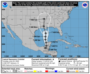
Three Oceans Under Cristobal

We have multiple ocean models in the coupled atmosphere-ocean hurricane forecast workflow:

1. The Navy Global Ocean Forecast System (GOFS3.1) – “It starts with us” to quote the Naval Oceanographic Command.  This is were the data assimilation takes place.
2. The NOAA global Real Time Ocean Forecast System (RTOFS) – derived from GOFS3.1 where the NOAA global winds are layered in.
3. Regional Hybrid Coordinate Ocean Model (HYCOM )- derived from RTOFS where the high resolution processes are layered in to properly respond to the intense hurricane forecasting.
4. Regional Princeton Ocean Model (POM) – currently initialized with climatology modified by feature models for the Loop Current and Eddies. Note that the climatology modified by feature models is scheduled to be retired July 1, 2020 and be replaced by an ocean derived from one of the RTOFS (items 2 or 5).
5. The NOAA global Real Time Ocean Forecast Model with Data Assimilation (RTOFS-DA) – this is the data assimilative version of RTOFS.  The Data Assimilation (DA) scheme is derived from the Navy Coupled Ocean Data Assimilation (NCODA) scheme, but some adjustments.  The biggest difference with NCODA is how altimetry is assimilated.  NCODA assimilates the altimetric sea surface heights by transforming them into temperature and salinity profiles using the Improved Synthetic Ocean Profiles (ISOP) and assimilating the synthetic profiles as “super obs”.  RTOFS-DA assimilates the sea surface height (causing a barotropic pressure change throughout the water column), then adjusts the isopycnal layer thicknesses (to adjust the baroclinic pressure) to produce no total pressure change at the bottom.  The result is that RTOFS-DA and NCODA (used in GOFS) have two different ways to adjust the subsurface temperature and salinity fields.  This is important because Argo floats provide us the large scale thermal and salinity structure of the ocean, the altimeter data layers in the Mighty Mesoscale, and the underwater gliders fly in to tidy up the fuzzy spots.  Three critical steps in our efforts to provide the hurricane models with the best representation of the ocean possible.  RTOFS-DA changes how we do the critical step of layering in the Mesoscale, making this an important piece of our summer research.

Now the important step, an ongoing collaboration between Maria at Rutgers and Hyun-Sook and Zulema at NWS. They are an awesome team dedicated to improving the ocean side of the hurricane forecast models. None of this would be possible if these three scientists were not actively collaborating and talking to each other multiple times a week.

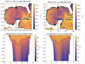
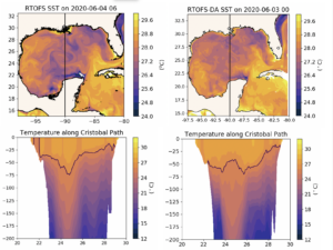
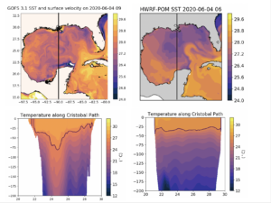
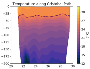
Maria has prepared two views of each of the different model oceans that were available for Tropical Storm Cristobal.  Each model is represented as a column in the figures.  The top row is a map of the surface temperature in the Gulf of Mexico immediately before the passage of Cristobal.  The bottom row is the vertical temperature section of the upper 200 m from south to north along 90W, the approximate track Cristobal was about to follow across the Gulf.

The first plot below compares GOFS3.1 (model 1-  where data assimilation takes place) with RTOFS (model 2- where nosaa winds are layered in).  As expected, the two models look very similar in both the map view and the vertical section.  The important feature is warm anticyclonic Loop Current Eddy centered at 25N, 9oW.

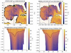
Next we move from the global RTOFS (model 2) to regional HYCOM (model 3).  Regional HYCOM is the ocean in the “Hurricanes in a Multi-scale Ocean-coupled Non-hydrostatic (HMON)”.  The US is required to operate two official hurricane models and HMON is one of them.  In the figure below we see that the regional HYCOM that HMON is coupled to looks very much like ROTFS which looks very much like GOFS.  This is the way the workflow is designed to work, – get the best available assimilation, get the best available winds, and get the ocean into the high resolution models we need – setting up the best initial condition for the ocean before the hurricane even enters the region.  HMON has the best ocean the Navy and NOAA – working together – can provide.

Now we look at the second of the two hurricane models, the Hurricane Weather Research and Forecast  (HWRF) model.  HWRF is one of the highest performing hurricane models in the global ensemble. In the Atlantic Basin, the ocean model that HWRF is coupled to is the Princeton Ocean Model (POM). The Princeton Ocean Model is not initialized using the GOFS to RTOFS to HYCOM workflow described above.  In the Atlantic Basin, it is initialized using climatology modified by feature models for the Loop Current and Eddies. Comparing the maps below, we see that the Loop Current is in the wrong location based on the satellite altimetry, and the Loop Current Eddy is not present at all.  The POM model under HWRF appears to be initialized by climatology only.

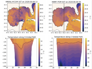
This is a significant dilemma.  One of our required hurricane models, HMON, is coupled to the best ocean Navy and NOAA can provide.  And our other hurricane model, HWRF, one of the global leaders in hurricane forecasting, is coupled to a climatological ocean that does not include the Essential Ocean Features impacting hurricane intensity.  We look forward to the next update of operational HWRF scheduled for July 1, 2020.

Enter RTOFS-DA (model 5 above). Can we reduce the distance between the data assimilative model and the regional scales we need to resolve the Essential Ocean Processes. RTOFS-DA is currently running at NWS in an experimental mode. In the figure below, we have the operational ROTFS in the left column and the experimental RTOFS-DA in the right column.  The Loop Current is a bit different, but not disturbingly different like it is in the climatology.  And both models have the warm anticyclonic Loop Current Eddy near 25N, 90W.  But there are differences in the eddy structure.  In the deeper part of the temperature section, say between 50 m and 200 m, the Loop Current Eddy is stronger in ROTFS-DA.  So at depth, one has a stronger eddy, one has a weaker eddy, but both have an eddy, so we are doing good.  But what about the upper 50 m.  Here we see differences in the structure of the eddy in the water warmer than 26C (the black line in the bottom row of plots).  The 26C isotherm domes up in the middle of the eddy like is does in a cold core ring with cyclonic circulation.  The impact on the surface map is we don’t see the swirling motion of the alternating bands of warm and cold water wrapping around the eddy due to the clockwise surface circulation that we see in RTOFS.  No this is an important difference for hurricane forecasting since it is the water above 26C that contributes to the calculated Ocean Heat Content (OHC).  And maps of the OHC are used by the forecasters at the National Hurricane Center to alert them to potential regions where hurricanes may intensify.  The operational RTOFS has a maximum in the Ocean Heat Content in the center of the Loop Current Eddy.  And the Experimental RTOFS-DA has a local minimum in the Ocean Heat Content in the center of the eddy.  These are two very different answers, and provide the NHC forecasters with very different guidance. So now we have work to do.   Which one is right and why?

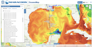
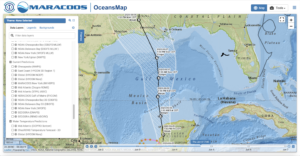
OceansMap view of Cristobal

Here are two quick views of Cristobal from OceansMap.

First we look at the  current position and track of Cristobal over the Navy GOFS 3.1 model forecast for today’s Sea Surface Temperature.  Cristobal is currently on the southern side of the Anticyclonic warm Loop Current Eddy. It will take most of today (Saturday) to cross over the eddy.  Official NHC forecast has the intensity at 40 knots. The forecast is for a slight increase in intensity by about 11 mph as it crosses the Gulf with landfall Sunday.

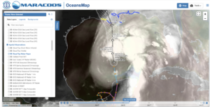
But Cristobal is a very broad storm as seen in the satellite cloud top water vapor product below, with the strongest convection to the north and east. The official NHC warnings extend well to the east of the expected landfall region.

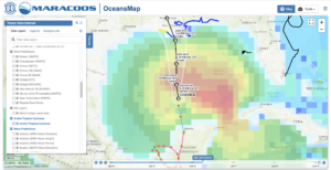
To get an idea of the scale of the impacts of this broad storm, we can check the global NOAA Wavewatch III model.  The modeled waves indicate that this is a full-Gulf event.

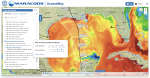
Two Different Oceans

Below is a side by side comparison of the two oceans we have been looking at for the last 24 hours.  The left hand column is the Navy’s data assimilative Global Ocean Forecast System (GOFS) 3.1.  Right column is the regional-scale Princeton Ocean Model (POM) initialized using Loop Current and Eddy features models to adjust climatology.  The top row is a map of the Sea Surface Temperature (SST).  The black line running south to north along 90W is the approximate forecast path of TS Cristobal.  Bottom row is the vertical temperature section along the 90W line between the surface and 200 m depth.

HWRF-POM initialized with climatology and feature models

The last few blogs talked about what we see in the Navy GOFS 3.1, the data assimilative step on the ocean side of the coupled atmosphere-ocean hurricane models.  My blog post from May 15, 2020 describes the multi-step process that gets us to the operational models.  GOFS3.1 is the data assimilation step.  This information flows into Global RTOFS to layer on the NOAA global windfields.   But remember, these both are global models, their job is through data assimilation and the good windfields to get the Essential Ocean Features in the right locations.  We then initialize a high resolution regional ocean model capable of resolving the Essential Ocean Processes that impact hurricane intensity during the rapid co-evolution phase of the atmosphere and ocean subject to intense hurricane forcing.

Another path to the regional scale ocean model underneath the hurricane is the feature model initialization process. Here climatology is modified by typical structural models for key Essential Ocean Features.  In the Gulf of Mexico, a forecaster provides 3 points to describe the location of the Loop Current, and the a model for a typical Loop Current is inserted.  For the warm eddies, climatology is modified by inserting bowl shaped structures to represent the warm core.

Here we investigate the results of that feature model initialization procedure used in the most recent HWRF-POM coupled forecast for Cristobal. The first image below is the Sea Surface temperature for  the POM ocean model coupled to the HWRF atmospheric model.  We see the Loop Current is present, but it looks to be shifted west of the Loop Current seen in the data assimilative GOFS or in the CoastWatch altimetry product.  It definitely is not up against the West Florida Shelf as it exits the Gulf.  Along the 90W line we have been talking about, the water is relatively warm on much of the Yucatan Shelf, with some upwelling occurring on the shelf.  But as you head north along 90W and leave the Yucatan Shelf, you encounter some of the coldest water in the Gulf.  The large warm eddy observed in GOFS and the CoastWatch altimetric product centered near 25N, 90W is absent from POM.

So lets layer on the surface currents to search for the structures in the current field.  The GOFS experience taught us that the SST may be confusing due to surface processes, and that the sea surface height and the surface currents are better for identifying the eddies.  Below is a plot of the POM ocean model SST and Surface currents. The Loop Current is certainly present, but the anticyclonic circulation we have been talking about since last night is absent.

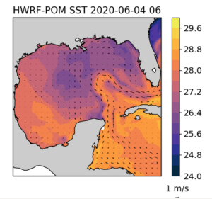
Ok, so lets just move straight to the subsurface section running from south to north along 90W.  There is no bowl shaped warm core ring in the temperature section running from the Yucatan Shelf to the Louisiana Shelf.  The 26C isotherm is pretty shallow, hovering around 30 m deep.  Also wondering where the continental shelves on the north and south are.  Looks like more to investigate.

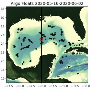
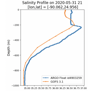
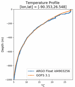
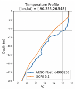
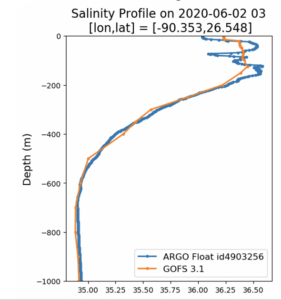
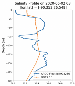
An Argo Float from the critical Warm Eddy

Here we look back on the Argo floats locations for the last 20 days.  Looking for one closer to the eddy center.  So we chose one near  25N, 90W.

For the temperature comparison, we see the near surface region is similar in magnitude but with multiple mixed layers in temperature in the Argo data. Profiles at the depths below 600 m are also similar, but the main warm core of the eddy between 100 m and 600 m is different.  Argo data is warmer than the model.  Perhaps this is a true temperature difference, or perhaps it is simply a difference in location.  That the real world Argo profile may be closer to the center of the eddy than the same location in the model.  To help answer this question, it is often good to look at the profiles relative to an eddy center based coordinate system.   We can do that in the model.  More difficult in the data when you only have a single float profile and you can’t direct the float into the eddy center.

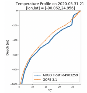
The same discussion applies to salinity.  The core of the anticyclonic eddy is warm and salty.  The Argo float is saltier than the model.  Maybe the Argo float is closer to the eddy center?  The Argo salinity profile also has a deeper mixed layer than the model.  Is this a difference in surface mixing?  or maybe it is part of the banding we see in the circulation around the eddy.   Easier to check in the model.  More difficult when you are dealing with a single profile instead of a cross-section through an eddy.

A quick check of the Satellite Altimetry

Here is my new favorite place to look for satellite altimeter products in the Gulf of Mexico, the NOAA AOML site:

https://www.aoml.noaa.gov/phod/dhos/altimetry.php

I have been a long term user of the CCAR altimeter products for the Gulf, but I am not seeing it.  Maybe our GCOOS friends have a recommendation for their go-to site for satellite altimetry.  Was very happy to find this CoastWatch site from our friends at AOML.  It has exactly the confirmation information we are seeking on the pre-storm ocean conditions.

In a previous blog post, we plotted the Sea Surface Height (SSH), and the surface currents, from the GOFS 3.1 model, noting that the Essential Ocean Features impacting hurricane intensity are well defined by SSH.  Below is the CoastWatch altimeter product that plots the SSH  (orange is high elevation, blue is low elevation) and the resulting geostrophic currents.  The Loop Current flowing into and out of the Gulf is on the lower right. Nearly centered at 25N, 90W, is the large, warm core, Loop Current Eddy that Cristobal is forecast to track across tomorrow.  Farther north and to the right of the forecast hurricane track is the Warm Eddy located just off the Florida panhandle continental shelf. In between the two warm, Anticyclonic eddies with the high elevations is the smaller area of low elevation associated with the cyclonic cold feature just south of the birdfoot.  We clearly see the impact of the satellite altimeter in the data assimilative GOFS model.

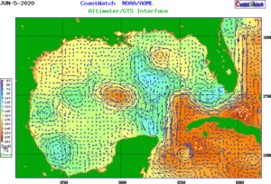
It looks like we are being given a well designed laboratory experiment with a tropical storm tracking directly over the center of a warm Anticyclonic ring.  Except that this one is real.

A next step will be to look for any of the operational regional HWRF runs that use the feature model initialization approach, and compare to the operational data-assimilative global GOFS model.

Argo Floats in the Gulf

National Hurricane Center forecasters still have Cristobal following the 90W latitude line north across the Gulf starting this weekend

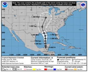
Here is a look at the Argo Floats in the Gulf that recently reported profiles between June 1-4. There are a couple near the north to south line along 90W.

Below is a quick look at the first temperature profile compared to the Navy GOFS version 3.1.  Everything below 200 m looks to be spot on.  Above 200 m the observed Argo profile is a bit warmer, with a deeper mixed layer.

Zooming into the upper 200m, we can see the details of the warmer ARGO profile.  Both have the same mixed layer temperature, but the mixed layer depth is less than 20 m and the argo float has it closer to 40 m.  Using the depth of the 26C isotherm as another metric, we see it is about 30 m depth in GOFS and about 55 m deep in the Argo data.

Now for the salinity comparison.  As with temperature, the salinity comparison between GOFS and the Argo Float look very similar.  In the upper 200 m, the salinity is much more variable.  So lets zoom into the surface layer.

Below we zoom into the upper 200 m. Here the big question is the barrier layer.  Temperature is nearly uniform down to a depth of about 50 m in the same profile, but the salinity profile indicates that there is a thin surface layer of  low salinity water that is uncorrelated with the temperature.  This is the critical barrier layer that inhibits mixing due to the resulting stratification.  If we only had temperature observations, we might assume that the surface mixed layer is unstratified, and free to mix with the cold water below. The good news is that we do see the lower surface salinity in the GOFS model, but in the model, the low salinity surface layer is about 20 m deep and the temperature mixed layer is about 20 m deep.  So the characteristics of the barrier layer are different.  Salinity and temperature are well correlated in the upper layer of model, and are independent in the upper layer of the data.

More comparisons to come as we work through the day.

Forecast Tropical Storm Cristobal

It starts with the National Hurricane Center, with a forecast track for Cristobal going up the Yucatan Peninsula, across the Gulf of Mexico and into the Gulf Coast.

I then turn to my favorite product visualizer, the MARACOOS OceansMap.  Below is a map of the forecast track for Cristobal over the bathymentry of the Gulf of Mexico.  Here we see that Cristobal is forecast to travel over the shallow Yucatan Shelf Saturday morning, then cross the very steep Campeche Escarpment into deep water.  Cristobal then spends Saturday afternoon through Sunday morning over the deep Gulf of Mexico.  On Sunday afternoon Cristobal starts making its way across the Louisiana – Texas continental shelf towards eventual landfall.

Next we use OceansMap to look for the Essential Ocean Features impacting hurricane intensity.  The Essential Ocean Features in the Gulf of Mexico are the very warm Loop Current, the warm and cold eddy features, and the fresh water from the Mississippi.  The Loop current enters the Gulf through the Yucatan Straits between Mexico and Cuba, forms and inverted U shaped loop inside the Gulf, and exits the Gulf through the Straits of Florida between the Keys and Cuba.  The largest Loop Current Eddies break off from the Loop Current and travel Westward across the Gulf through the deepwater region noted above. Below we look for these Essential Ocean Features using OceansMap.

In OceansMap we first bring up the Navy Global Ocean Forecast System version 3.1, based on the HYCOM model.  This is the model that assimilates all the ocean data for the hurricane forecasts, making it the critical first step in getting the ocean right. The nice thing about OceansMap is that the images can be manipulated in my web browser, so I can vary the enhancement.  Below we have plotted the GOFS 3.1 Sea Surface Temperature field and adjusted the color bar to highlight temperatures between 20C (blue) and 30C (red). The warm Loop Current is easy to see entering the Gulf, extending somewhat less than half way north, and sharply turning back south, running along the West Florida Shelf to exit through the Florida Straits.  We then move to identifying the eddies in our census of Essential Ocean Features.  The most critical are known as Anticyclonic Eddies due to their clockwise circulation patterns.  They are also known as Warm Eddies, since they have a deep warm subsurface structure that we don’t see in these surface maps, and warm water is the fuel for hurricane intensity.  Looking for regions of clockwise circulation we see two, one large area right under the forecast track of Cristobal.  Cristobal is forecast to be over this warm water feature Saturday 1 pm to Sunday 1 am.  This is the location to watch.  The other clockwise circulation feature is to the right of the storm track up against the West Florida Escarpment.   The next set of Essential Ocean Features are the Cyclonic Eddies, with counterclockwise circulation and a subsurface structure that is cold. The cold water in these eddies have the effect of trying to weaken the storm.  One of these Cyclonic Eddies are located just south of Louisiana birdfoot, between the two Anticyclonic eddies noted above.  There also appears to be very cold upwelled water on the shallow water of the Yucatan Shelf, and in the shallow water of the West Florida Shelf.

The OceansMap view of the Essential Ocean Features in the Gulf of Mexico prompts us to look deeper into Navy GOFS 3.1 model.  Below are plots of the temperature (top row) and salinity (bottom row) from GOFS model on June 4, 2020.  Surface values are on the right column and values at 200 m depth are in the left column.  For surface temperature (upper right) the features seen in OceansMap are reproduced. They include the Loop Current, the two Anticyclonic eddies, and the one Cyclonic eddy in between.  Looking at the temperature at 200 m depth, a depth below the seasonal thermocline, we see these features are well defined by their temperature structure. The anticyclonic eddies defined by their circulation at the surface are well defined by their warm cores.  The cyclonic eddy is well defined by its cold core.

Now we look at the salinity in the bottom row.  The surface salinity shows us the location of the Essential Ocean Features called barrier layers. These layers are barriers to mixing and enable the ocean to stay warm longer, contributing more to the intensification of the hurricane than it would if no barrier layer was present. In this view of the surface salinity, we see the Mississippi River plume and how it is spread along the Louisiana-Texas continental shelf.  At 200 m, below the seasonal thermocline & halocline, the subsurface salinity map highlights different features than in the surface map. The large scale Loop Current and Eddies that we see in the 200 m temperature layer are reinforcing the way we define the anticyclonic eddies – that they have warm, high salinity waters that extend well below the surface.

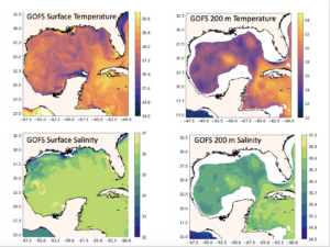
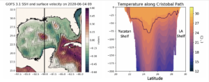
Below we look at a map of the sea surface height (SSH) on the left.  The surface circulation we are using to define the Anticyclonic and cyclonic eddies is related to the variations in sea surface height.  Anticyclonic circulation occurs around a high (red color) in the SSH. Cyclonic circulation occurs around the low elevations (blue) in the SSH.  The eddies are very visible in the SSH fields, which illustrates the importance of the satellite altimeters to define the Essential Ocean Features in the Gulf of Mexico.

On the right we show a vertical temperature section running from south to north along 90W marked by the black line in the SSH map.  In the vertical temperature section, the 26C isotherm is marked by the black line. In this case, 26C is also near the base of the surface mixed layer.  The 26C isotherm is typically 25m to 40 m deep, except within the warm core ring, where the 26C isotherm extends to a depth of about 80 m.  We also see that most of the variability in the model is in the upper 100 m. At about 200 m, the water is relatively cool except for the warm water in the core of the ring.