SEAB Results

The following figures were generated using data collected from the 13 Mhz Sea Bright (SEAB) site. This data was collected on November 9th, 2009.

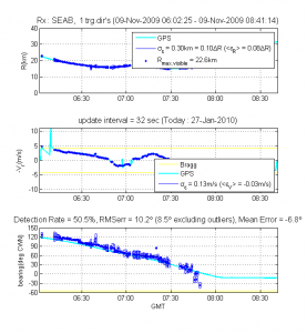
For this experiment, the Los Angeles tanker ship was selected to be tracked. This plot contains three graphs. Each graph contains the ship’s GPS Tracks.  The first graph is Range vs. time. The second is Radial Velocity vs. time. The third graph is bearing vs. time. Using the median method (FFT: 128, Threshold- 8 db) for detection, the highest detection rate for the Los Angeles was 50.5%. As you can see, the SEAB HF Radar site detected the Los Angeles fairly accurately. From the second plot, we can see that the Los Angeles traveled in between the Bragg peaks the entire time.

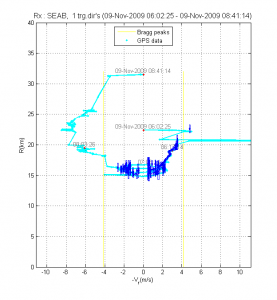
A Range (km) vs Radial velocity (m/s) graph depicting the GPS track of the Los Angeles and the detections of the ship from HF Radar. The ship was in between Bragg peaks almost the entire time.

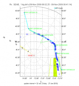
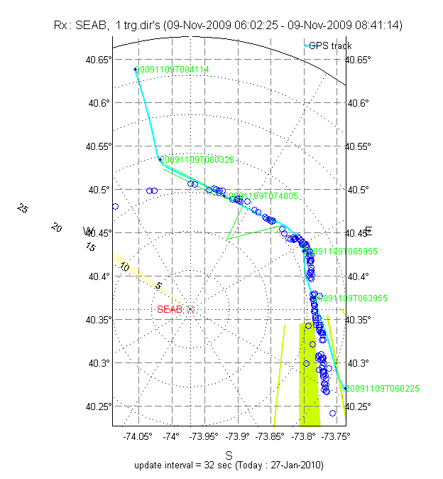
A coordinate map depicting the GPS track of the Los Angeles. The detections done by the SEAB site are the blue circles laid over the track. As you can see, the GPS track and HF Radar Ship Detection match up quite well.

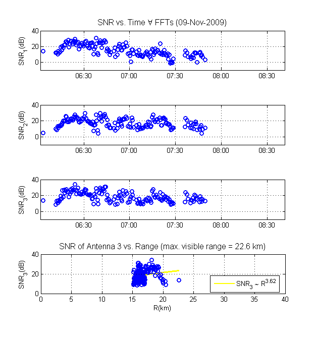
Signal-to-Noise ratio vs time plots: The first graph is the SNR from Loop 1,  the second from Loop 2, and the third from the monopole. The fourth graph depicts the SNR from the monopole vs. range.  The shipping lanes are approximately 10 and 20km from the New Jersey coastline. This is why there is no SNR from to 15km.

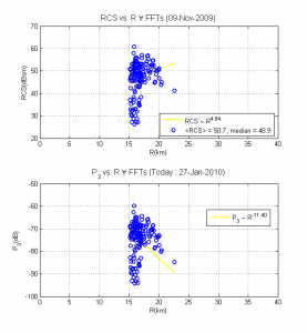
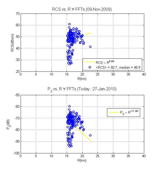
RCS vs. Range

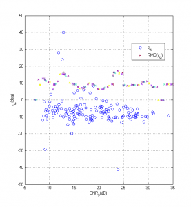
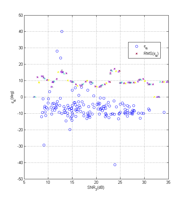
Degrees vs SNR (Monopole).