LEAP Performance Report response

Hugh,

I decided to pick these vessels, because the Orange track has an interesting track, just moving outside of Barnegat. Sometimes ship detection notice some interesting boats just hanging out. The darker blue and green track I choose because there are some instances where the detection have some gaps. Both ships have similar radial velocity and distance, but different bearing. I am curious on how would the code resolve the differences, and see how it does with the gaps. The yellow track seems to be a straight line down south on the map, however, on the second graph, the vessel shows gradual change in distance to the radar as well as in bearing. Seems interesting on how the vessel moves. If you, see other vessels that need to be included please let me know.

LEAP Performance Report

Erick, how did you decide that you’ll plot 7 ships?  Can you plot them all?

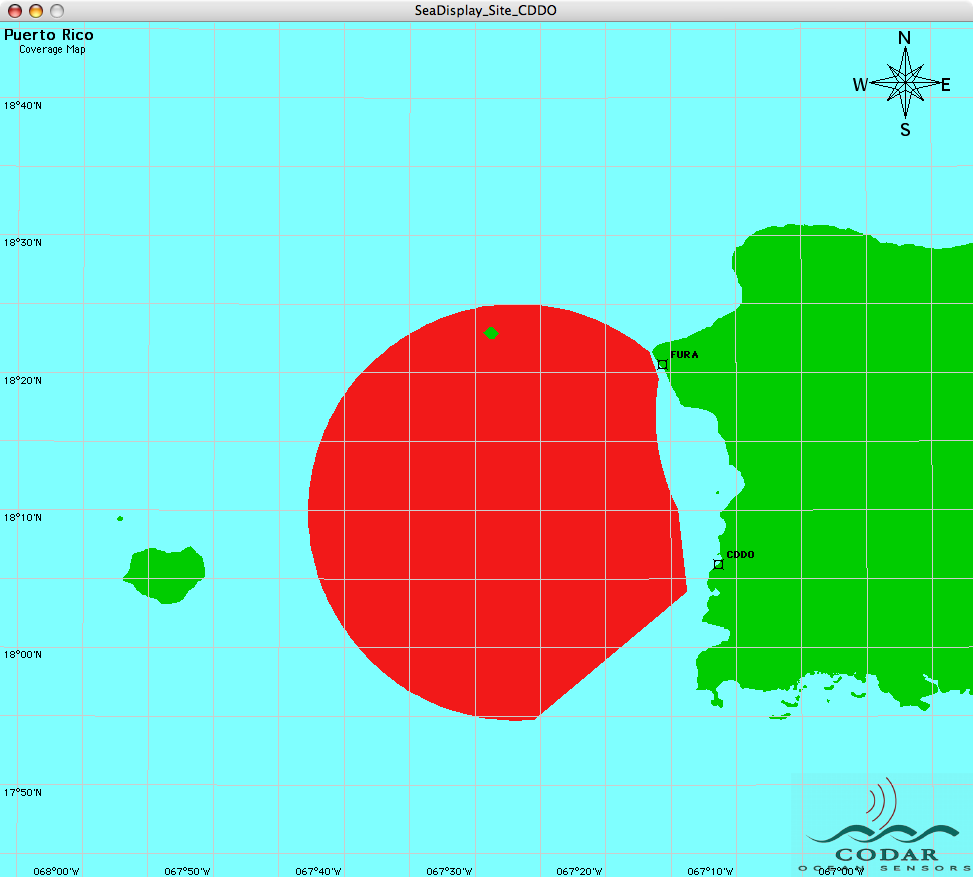
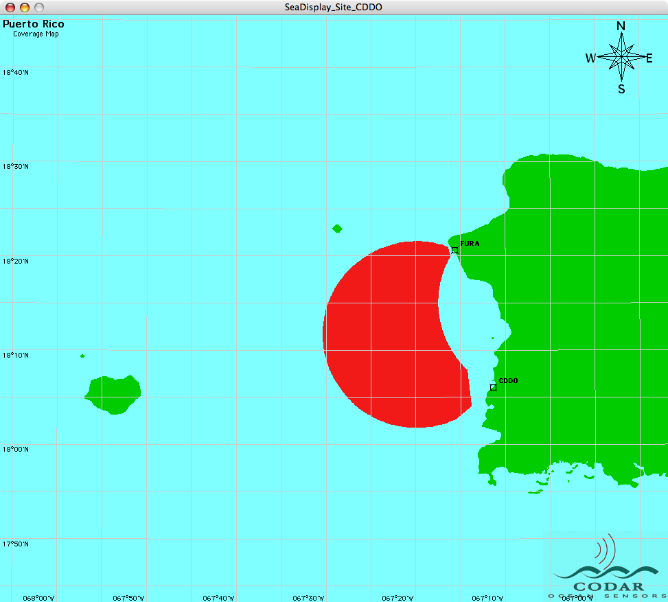
Stability Angles and Coverage at the FURA and CDDO sites

The following are hypothetical coverages associated with the FURA and CDDO sites that are run by the University of Puerto Rico – Mayaguez. Each plot was made by changing the Stability Angles. As the stability angles are increased, the total coverage of the two sites decreases.

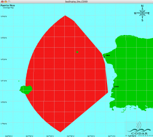
This picture is when the stability angles were set to 10.

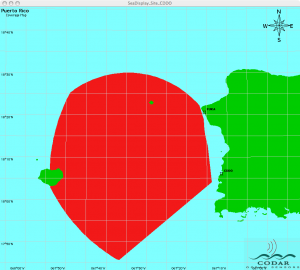
Stability Angles: 20

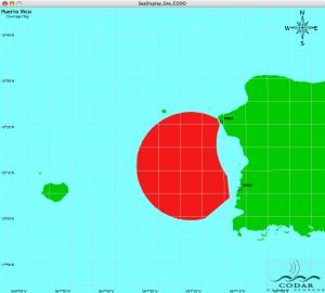
Stability Angles: 30

Stability Angles: 40

Stability Angles: 50

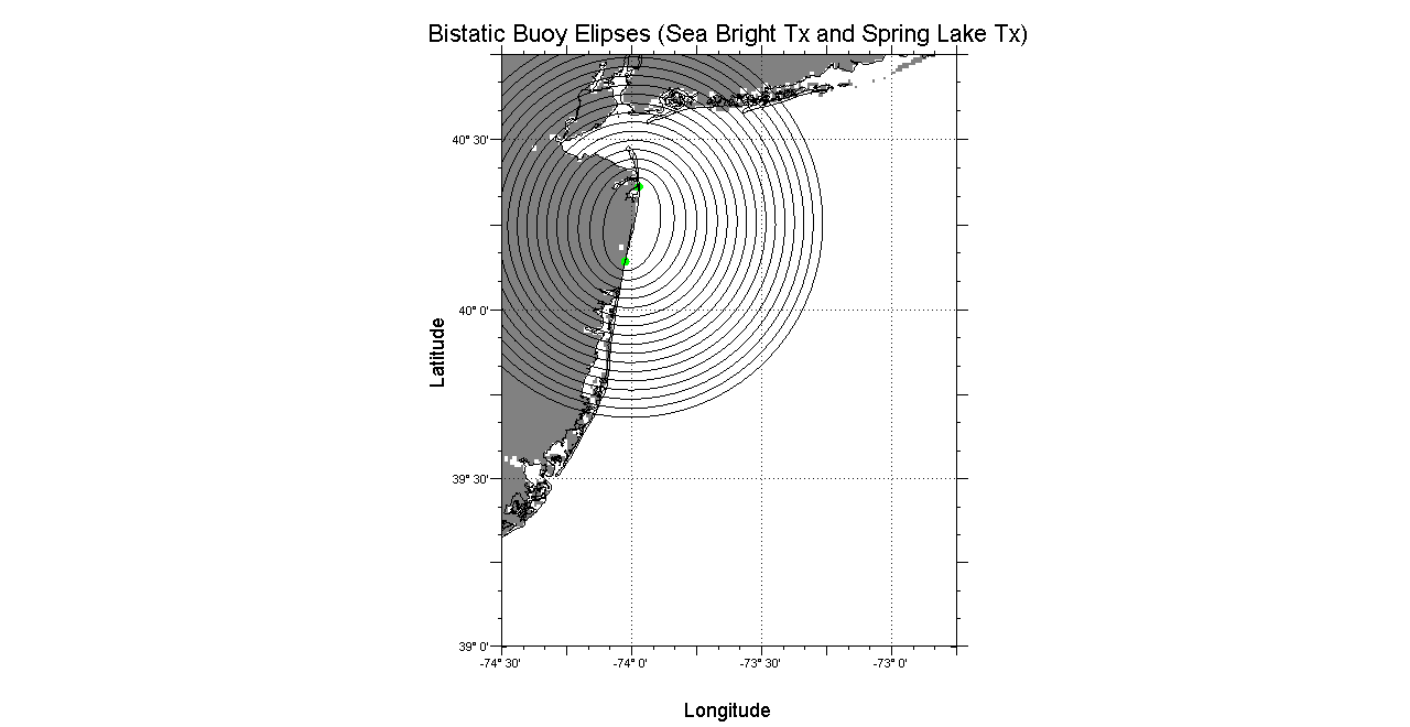
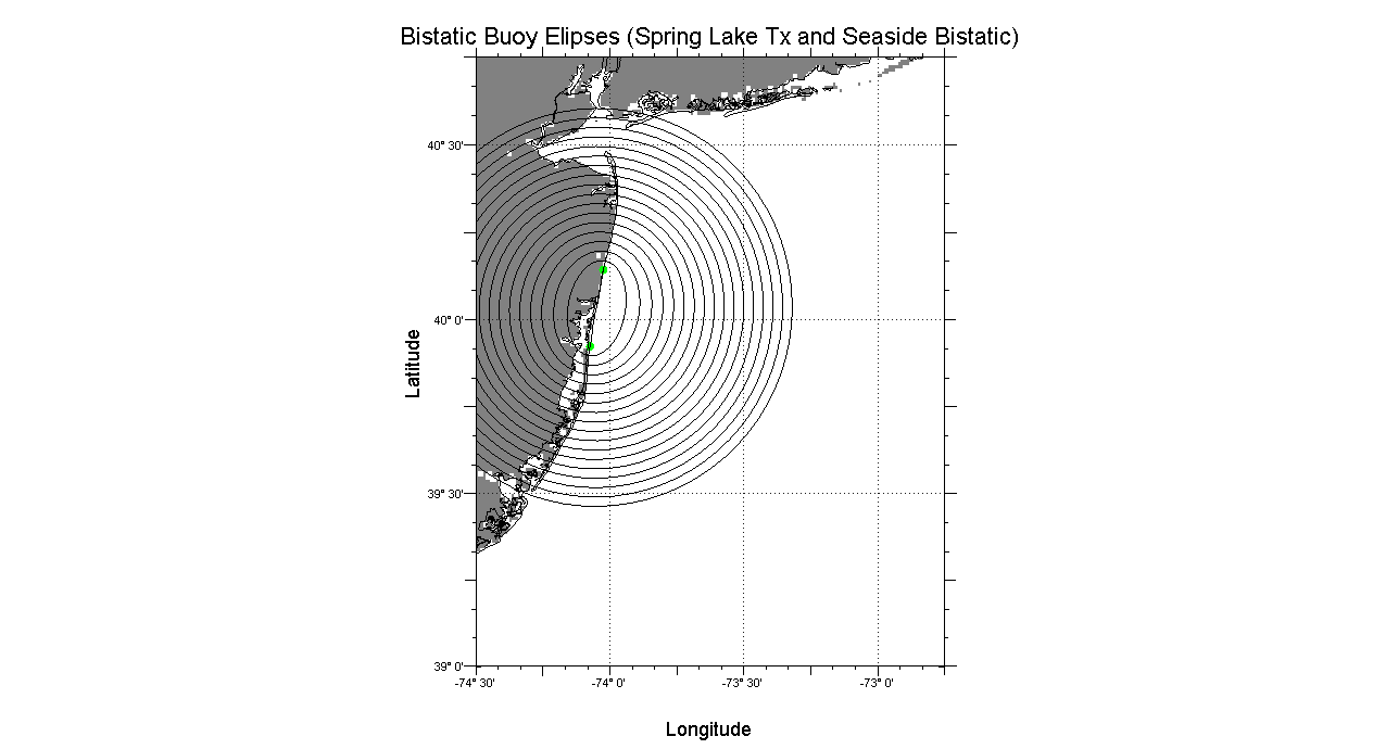
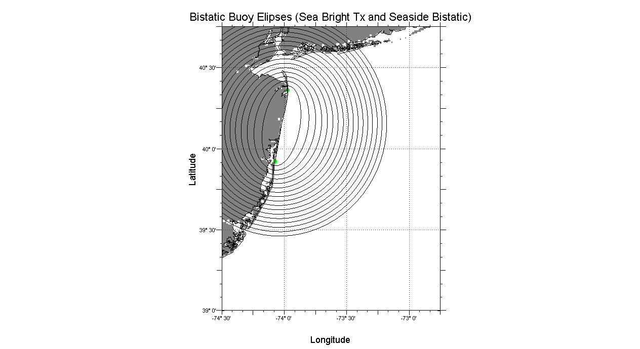
Bistatic Ellipses between Sea Bright Tx and proposed sites in Seaside and Spring Lake

Here are some plots that I created that estimate bistatic ellipses between our Sea Bright Tx site and the proposed Spring Lake Tx and Seaside Bistatic sites.

Sea Bright Tx and Spring Lake Tx Ellipses

Proposed Spring Lake Tx and Seaside Bistatic Transmitter Ellipses

Sea Bright Tx and Seaside Bistatic Transmitter Ellipses

SEAB Results

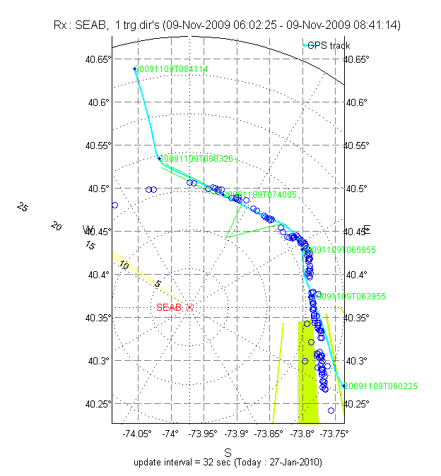
The following figures were generated using data collected from the 13 Mhz Sea Bright (SEAB) site. This data was collected on November 9th, 2009.

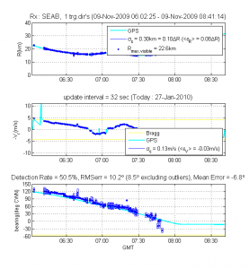
For this experiment, the Los Angeles tanker ship was selected to be tracked. This plot contains three graphs. Each graph contains the ship’s GPS Tracks.  The first graph is Range vs. time. The second is Radial Velocity vs. time. The third graph is bearing vs. time. Using the median method (FFT: 128, Threshold- 8 db) for detection, the highest detection rate for the Los Angeles was 50.5%. As you can see, the SEAB HF Radar site detected the Los Angeles fairly accurately. From the second plot, we can see that the Los Angeles traveled in between the Bragg peaks the entire time.

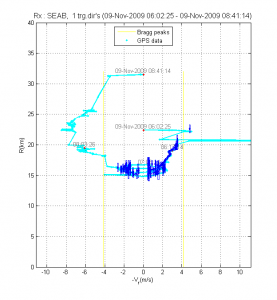
A Range (km) vs Radial velocity (m/s) graph depicting the GPS track of the Los Angeles and the detections of the ship from HF Radar. The ship was in between Bragg peaks almost the entire time.

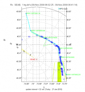
A coordinate map depicting the GPS track of the Los Angeles. The detections done by the SEAB site are the blue circles laid over the track. As you can see, the GPS track and HF Radar Ship Detection match up quite well.

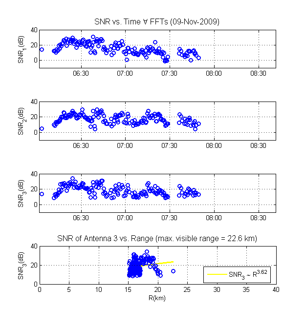
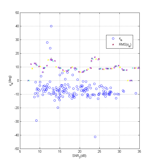
Signal-to-Noise ratio vs time plots: The first graph is the SNR from Loop 1,  the second from Loop 2, and the third from the monopole. The fourth graph depicts the SNR from the monopole vs. range.  The shipping lanes are approximately 10 and 20km from the New Jersey coastline. This is why there is no SNR from to 15km.

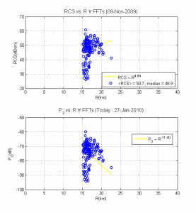
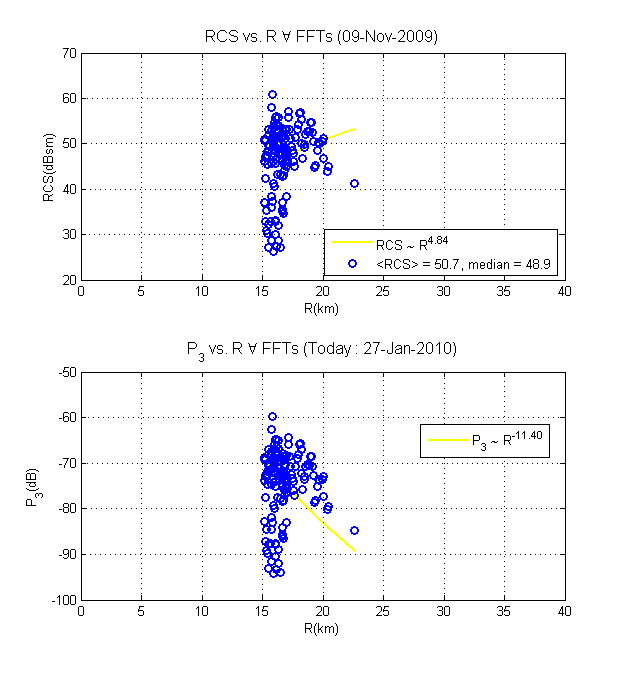
RCS vs. Range

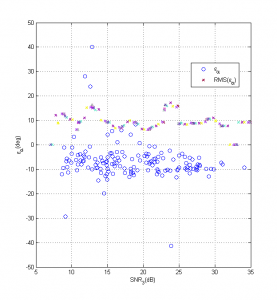
Degrees vs SNR (Monopole).

AIS Data from Monday

Eric converted the AIS data from Monday November 9.

the ‘rLOVE_AIS’ contained        23,874         data points or 19% of the data

the ‘rSandyHookNOAA’  contained 4,031 data points or 3% of the data

the ‘rTuckerton’ contained 98,935 data points or 78% of the data

Detections towards end of Day 1

HOSR detection at 14:55

HOSR detection at 13:33 GMT

SILD detection at 13:20 GMT